1. Intro
TL;DR: I wanted to see what would happen if I gave an LLM direct control of my oscilloscope to help me decipher waveforms from a Class D amplifier in my kids’ audiobook player, and ended up with a general tool that’s helped me blind-characterize two power supplies from ripple alone, decode an unknown UART stream from raw analog samples, and find broken firmware commands. Code and raw data are here.
Disclaimer: I slept through two years of electronics in my CS degree, and my practical skills topped out at Ohm’s law. But I promised myself that if I ever took a break from work, I’d have a stab at electronics again. This has been mostly a way to improve my basic signal analysis techniques, and fix a few broken toys around the house.
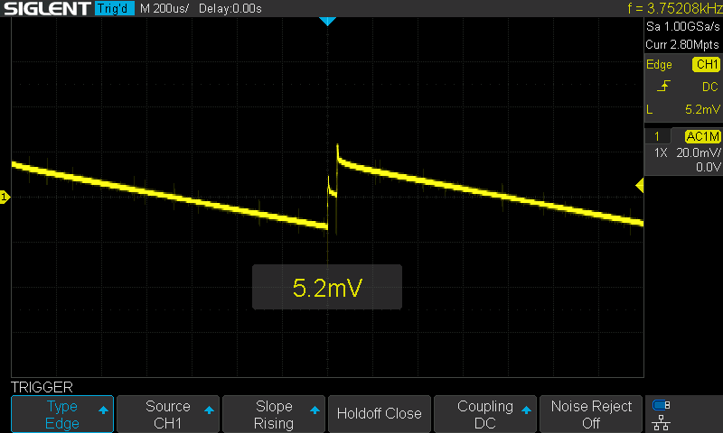
Figure 1: A USB PD charger’s output ripple, captured and identified by an AI driving the scope over the network. The textbook PFM sawtooth — slow capacitor discharge, then a burst of switching pulses — was found without any hints about the hardware.
2. Setup: giving an LLM hands, not a brain
After figuring out that my Siglent SDS1104X-E could be controlled by commands over TCP/IP, I wanted to see how far the LLM could take it in figuring out the rest of the commands, and come up with a bare bones API to control it. I gave it the model of the scope, and gave it a sample of what worked:
$ echo "TDIV?" | nc -w 1 scope.quesejoda.com 5025
TDIV 2.00E-05S
Claude’s first instinct was to expose everything: every SCPI command the scope supports, wrapped in its own function. This had a very bad smell. A human using a scope only touches a handful of things: set the channel, set the timebase, set the trigger, take a measurement, grab waveform data, etc. I deliberately kept the higher level functions out: the scope’s built-in FFT, math channels, and protocol decoders. If Claude needed to analyze a signal’s frequency content, it could download raw samples and run numpy. If it needed to decode a protocol, it could look at the bits itself.
I pared down the API to a bare minimum, and the result was a single Python file with a handful of tools covering scope configuration, measurement, waveform capture, and a screenshot function that lets the model literally see the scope display.
3. Finding firmware bugs the hard way
First, I designed a test harness that the AI could use to double-check its work against a known source, basically a Raspberry Pi acting as a signal generator for various square waves. I wrote some unit tests stressing the API, and I sat back. The result was rather surprising — the agent iterated for a while, tweaking timing issues and relieving me of the most boring parts. But interestingly, on the first run, it found two firmware bugs.
TRIG_STATUS? and the hallucination that looked real
Before this project, I’d been exploring the scope’s SCPI interface with ChatGPT, because I had no idea where to start. It suggested TRIG_STATUS? to query the trigger state and the scope diligently responded with TRST OFF which seemed perfectly reasonable. I included it in Claude’s project prompt as an example of a working command.
The problem is that TRST OFF is all it ever says. Running, stopped, triggered — always OFF. Apparently, after some digging I found that the command exists in the LeCroy vocabulary (from which the SDS1104X-E descends), but on this Siglent firmware it’s a stub that returns a syntactically valid response meaning nothing.
Claude found the working alternative, SAST?, by trying commands until it could set a trigger and read back the trigger status. I marked the “bug” as interesting and decided to investigate it myself. However, when I went looking for TRIG_STATUS? in the Siglent docs, I couldn’t find it anywhere. After doing some archeology through my notes, I noticed the command came from a ChatGPT session where I was trying to figure out how to talk to the scope.
Interestingly, the agent built an entire scaffold around a broken command, or rather a syntactically perfect entry point which was semantically empty.
For the curious…
Reproducing the bug (SDS1104X-E, firmware 8.3.6.1.37R17):

$ echo "TRMD AUTO"    | nc -w 1 scope.quesejoda.com 5025
$ echo "TRIG_STATUS?" | nc -w 1 scope.quesejoda.com 5025
TRST OFF              ? always OFF, regardless of state

Working alternative:
$ echo "SAST?"        | nc -w 1 scope.quesejoda.com 5025
SAST Auto             ? actual acquisition state
MSIZ is silently ignored
MSIZ 7K (sets the memory depth to 7,000 points) returns OK but the readback always shows MSIZ 14M, or whatever the scope’s memory depth happens to be (manually) set to. I tried every size, trigger stopped and running, no difference. The command is accepted without error and does nothing. The workaround is to set the memory depth manually on the scope.
$ echo "MSIZ 7K" | nc -w 1 scope.quesejoda.com 5025
$ echo "MSIZ?"   | nc -w 1 scope.quesejoda.com 5025
MSIZ 14M         ? unchanged, regardless of value sent
4. Making an LLM fall on its face deciphering a 1 kHz square wave
Early on, I clipped the probe to the scope’s own calibration terminal — a 1 kHz, 3 Vpp square wave that anyone can recognize on sight. I asked Claude to identify the signal.
It grabbed 2,000 raw samples. At 1 GSa/s, that’s 2 microseconds of data — 0.2% of one cycle. Every sample read ~3V. Conclusion: “DC rail, no signal.”
I told it to try harder. It grabbed 50,000 samples from three positions. Each 50 us window — still 5% of a cycle — landed in the same flat portion. It wrote a full analysis suite: FFT, autocorrelation, histograms. Everything confirmed flat DC with quantization noise.
I figured this was going nowhere fast, a failed experiment to archive, along with my other ones. But I poked the agent with “I see a square wave on the screen.”
It finally did the arithmetic. At 1 GSa/s, one period of 1 kHz is 1,000,000 samples. It grabbed five small windows spaced at half-period intervals and saw the alternation: 3V, 0V, 3V, 0V, 3V. Signal identified.
Post-mortem, I asked the LLM what would have made its life easier, and without skipping a beat it said… “a way to look at the screen” :-). Fair enough.
This was the most productive failure of the project. It led directly to three improvements: a screenshot tool, a time-aware waveform capture tool (so you ask for “10 ms of data” instead of “50,000 samples”), and a signal summary tool that auto-ranges before measuring: not terribly different from what a human would do.
The screenshot tool was transformative, but it took a few tries to get right. I noticed the AI could figure stuff out quicker, but still spectacularly slow, until I realized that the BMP coming from the scope was gulping up the entire LLM context.
Basically, the scope sends raw 16-bit BMPs; base64-encoding one consumed nearly a third of Claude’s context window. Converting to PNG server-side (62x smaller) and returning a file path fixed it — about 1,100 tokens per screenshot, conveying more information than any number of scope_measure calls. After adding it, Claude’s first move on any new signal was to take a screenshot, and then reaching for the measurement buttons: exactly like a human would do.
5. Blind power-supply characterization
With the basic infrastructure in place, I connected a power supply to the scope and told Claude to figure out what it was. No labels, no model numbers — just voltages on the probe. It did surprisingly well.
A bench supply reveals its switching modes
The first test subject was my cheap adjustable bench supply set to 2.5V. DC coupling showed a rock-solid flat line. AC coupling with the vertical scale cranked to millivolts revealed 18 mV peak-to-peak ripple.
The scope’s edge-based frequency counter was useless here: it reported 17, 31, 82, 127, and 774 kHz on consecutive captures of the same signal. Broadband switching noise has no clean repeating edge for the counter to lock onto.
Claude downloaded 50,000 raw samples, ran a Hann-windowed FFT, and found a clean harmonic comb at 21.5 kHz intervals, with no mains-frequency content. It correctly concluded that it was a switched-mode supply, not linear. Score!
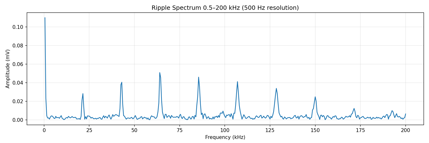
Figure 2: The software FFT that the scope’s edge counter couldn’t match. A clean harmonic comb at 21.5 kHz intervals — PFM burst-mode switching, visible out to the 9th harmonic.
Then I added load resistors. At no load, the ripple was the quiet PFM comb shown above. At 53 mA the spectrum spread out but stayed low. At 246 mA, a dominant peak erupted at 236 kHz, dwarfing the rest of the spectrum, and the LLM correctly concluded that the controller had switched to continuous PWM mode. It took the following image as part of its analysis (as well as the rest of the labeled images in this post).
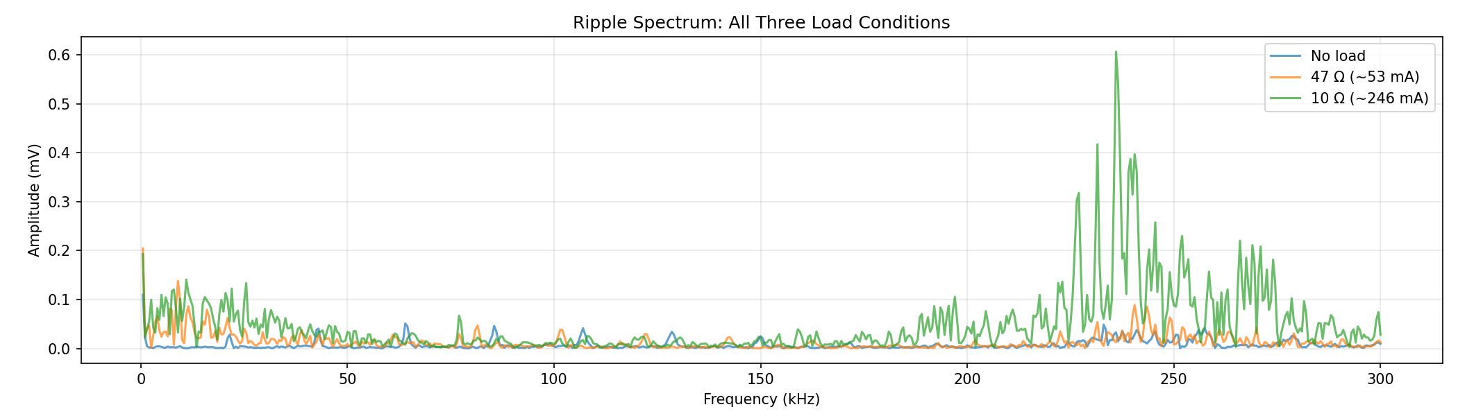
Figure 3: Adding load transforms the spectrum. The green trace (246 mA) shows a 236 kHz PWM peak that towers over the quiet no-load and transitional spectrums.
After the analysis, I revealed the PSU: a Jesverty SPS-3010V. The PFM-to-PWM transition, the 236 kHz switching frequency, and the 0.81% load regulation all matched what you’d expect from a modern buck converter IC with automatic mode switching.
The second subject — a budget 30W USB PD charger — told a different story. Where the bench supply transitioned cleanly from PFM to PWM under load, the charger stayed in burst mode at every load up to 1.2A, nearly half its rated power. Claude spotted a 680 Hz harmonic comb in the long-capture FFT — the burst repetition rate — and predicted it should be audible. Sure enough, the charger has an annoying hum you can hear in a quiet room. Same methodology, different topology, correctly identified from ripple alone.
6. Blind UART decode from analog samples
For the acid test, I connected a Raspberry Pi running a bit-bang UART script to the scope and gave Claude this prompt:
There’s a 3.3V microcontroller connected to CH1 that will send a short burst of digital data when I trigger it. I don’t know the protocol, baud rate, or encoding — just that it’s digital.
Set up the scope to capture the burst, then figure out what the data says.
The agent configured the channel for 3.3V logic, set a wide 70 ms window, and armed a single-shot trigger at the midpoint voltage. Three API calls. I fired the signal; Claude confirmed the capture; it took a screenshot to see the shape, then downloaded the full waveform.
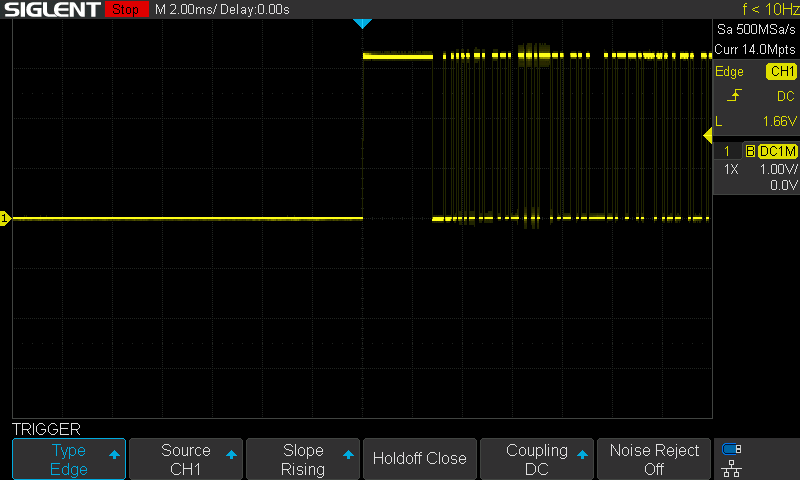
Figure 4: The captured UART burst. Idle LOW, a 3.3V preamble, then six bytes of data with visible bit transitions — all from a single-shot trigger.
Baud rate identification was immediate: “pulse widths clustered at exact multiples of 104 microseconds. 104 us = 9600 baud. The distribution is textbook: 14 pulses at 1x, 9 at 2x, 2 at 3x — integer multiples of a single bit period.”
Framing took a few passes. The line idled LOW instead of the standard HIGH (the MCU only enables its UART peripheral for the duration of the burst), which caused initial confusion about polarity. Claude resolved it by trying both interpretations and checking stop bits: only one polarity produced valid 8N1 framing on every byte. Six bytes decoded: dib$B\n (hex 64 69 62 24 42 0A). Correct.
The full decode — from “there’s a signal on CH1” to “it says dib$B\n at 9600 baud” — took about five minutes in a single unassisted run. Not instant, but faster than me trying to figure out bits from a screenshot. The methodology felt sound: capture wide, download everything, let the data tell you what it is.
Conclusion
One unexpected benefit: it’s become a decent scope tutor. I’m getting surprisingly competent instructions fro asking it: “I’m trying to scope X: set the scope up, and tell me what you did step by step”: Appropriate scales, plausible triggers, and adjustments based on what it sees on screen. After all, I want to improve my electronics-fu, not have the bot take over the fun parts :).
The division of labor ended up feeling natural: the AI handled the tedious parts (writing SCPI wrappers, debugging timing races, laying out Makefile targets) while I did the interesting parts (choosing what to expose in the API, connecting probes, placing load resistors). Nothing in the tool interface needs to change when the signal does — and that’s the point: just a handful of basic tools covering any analog or digital signal.
The project is open source under the MIT license: github.com/aldyh/pacoscope. The repo includes the MCP server (Model Context Protocol — how the LLM calls external tools; ~900 lines of Python), a Raspberry Pi signal generator, hardware-in-the-loop tests, the original prompts, and all raw data, plots, and scope screenshots from the PSU analysis.